
Release version v1.0.0
Release version v1.0.0
An online platform for African wetland and waterbird data

The BIRDIE project gathers and interprets data about wetlands and waterbirds to provide information that is useful for decision making. It sources data from citizen science databases, which are checked and analysed using statistical models. An online dashboard lets users access up-to-date indicators about bird distribution, abundance and richness at wetland sites. The information can be used for reporting, management, research and as a resource for birders. Find out more in About
BIRDIE is only for waterbirds, and currently there is no plan to develop the project for non-wetland birds. The main reason is that there is no count data for non-wetland birds like the data collected by the Co-ordinated Waterbird Counts (CWAC). Information on waterbirds is also much needed for reporting on South Africa’s international commitments to wetland and waterbird conservation. There is still much work to be done on BIRDIE, so our focus remains here.
The best way to contribute to BIRDIE is by continuing to support and take part in the Coordinated Waterbird Counts and the South African Bird Atlas project . The data collected in these projects feeds into BIRDIE. Ensuring these citizen science projects are ongoing and improving helps the continuation and development of BIRDIE. BIRDIE does not replace these projects – it uses the data collected to help inform decision making.
If you would like to suggest a wetland site to be added or have information on a site, please contact the Coordinated Waterbird Counts team to add a site to their database, where information can be collected bi-annually.
There is always a version code on the BIRDIE page. This is because we want to keep track of when changes happen in BIRDIE and what those changes are. We follow regular programming conventions where we have "major.minor.patch". So version 1 would be v1.0.0. Then, fixes and patches would increase the last digit (e.g. v1.0.1). New features and database updates would increase the second digit (e.g. v1.1.0). Major changes that affect existing functionality importantly would increase the first digit (e.g. v2.0.0). For more information refer to https://semver.org/.
In principle, we plan to update our database and website with new information which includes any new sites or updated information once a year. This would translate into minor version updates. We have plenty of exciting ideas to include additional functionality into BIRDIE, although it is difficult to put dates to these. We are still busy making the first phase of BIRDIE as neat as possible.
If you would like to provide any feedback and suggestions, including any updates on information or corrections, please use the  button on the top of the website.
The interactive map viewer is the DIY (do it yourself) centre at BIRDIE. It allows you to freely explore indicators for the different species and sites covered by the project on an interactive map.
To navigate to the map viewer, select the  button from the home screen. The interactive map viewer will open in a new tab.
The selection menus on the left,  and
and  , allow you to select the indicators you might be interested in from the three currently available options: abundance, distribution and richness.
To show or hide layers on the map, click on the desired layer under the options. The icon  located in front of the name will change to
  once the layer has been selected. To remove a layer from the map, click on the name again or you can select the
  icon.
icon.
To have a bigger view of the map on the screen, the user can collapse the side panel. Do this by selecting the ![]() icon at the top of the layer side panel.
icon at the top of the layer side panel.
In addition, it is possible to change the display order of the different layers. Click on  in the open layer and drag it to the desired order. Note that the layer at the top of the list will be displayed at the forefront on the map.
Then, you can find sites and species of interest by applying certain filters. Filters can be geographic, such as provinces, or ecological, such as waterbird feeding guilds, and others. Use the drop-down menus under each heading to filter the information that you are looking for and selecting the  button. This button must be selected.
To select multiple species click on one species with your mouse, press ‘ctrl’ on the keyboard and then select another species. Up to five different species can be selected.
Once the request is processed, information will appear on the map. You will see either circular markers corresponding to wetland sites where the selected species have been detected or a grid of 5’ x 5’ cells (pentads) with information about the probability that the species is present in each of them.
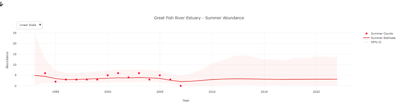
Once the abundance layer has loaded, you can then select a site  to see how the species abundance have changed over time on a graph. If you had selected multiple species, the plots will show a combined result for all the selected species.
Example of abundance graph that appears after clicking on a site.
The Sites and Species pages contain information that has already been analysed for you. Here you can get some deeper insights into species, site or programme indicators. The Sites and Species pages contain mainly summary tables. Therefore, the information is more readily usable by managers and decision makers.
You can go to the Site and Species reports by clicking on the  button. From here you can then choose either the Sites or Species buttons. Once there, you can choose the Site or Species that you are interested in by using the drop-down menu
 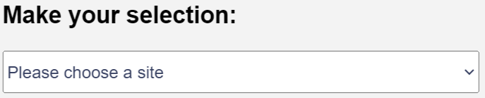 . There will be a ‘spinner’
  indicating that the site is busy loading. Once this has disappeared, the information is ready.
Sites and Species pages show changes in abundance across sites or species, as well as changes in species distribution. These pages also display important characteristics of sites and species related to their conservation status and threats.
There are multiple tables with information on BIRDIE. Most of the table are static. However, the bird information table on the Site pages and the abundance tables on the Species pages can be filtered and ordered.
You can interact with these tables by using either the search box  to search for a particular species, or using the drop-down menus below each heading to filter according to the information you are interested in.
Note: Once you select a filter, subsequent filters will be applied to the subset of information already filtered. Remove previous filters by changing the selection to blank.
You can order the data sets by selecting the  button. To revert the change, select the button again.
You can select the number of bird species you want to see on a page by selecting the drop-down menu 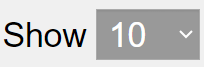 . Alternatively, you can go to the next page by using the page selection numbers
  below the table.
BIRDIE features bar plots showcasing the area of occupancy (AOO) and total population estimates at CWAC sites (per province) for each selected species. These plots are conveniently located on the Species page and are dynamically generated based on your species selection. Within the Exploration Map, trend plots come up when you click on a particular species at a site that show changes in abundance over time.
In all these plots, you have access to basic functions that enhance interaction. Next to the plot, you will find buttons for actions  such as downloading the plots as a PNG image, zooming in and out, panning, box selection, lasso selection, autoscaling, and resetting axes.
You can also hover over individual bars on the plot to view precise values for each year. You can click and drag the axes to change the display. These feature gives you a more detailed insight into the data presented, to better understand the trends and patterns over time.
You can download the maps, tables and plots that you have generated in the BIRDIE website.
Tables can be downloaded to an Excel spreadsheet by selecting the  button below the table.
Maps can be downloaded by clicking on the  on the map viewer.
Plots can be downloaded by clicking on the  on the graphs.
The Exploration Map includes ways to explore, interact with and filter bird indicators and ancillary data layers on a map.
The bird indicator layers include:
In addition to bird indicators, the Exploration Map also displays some environmental data layers that are relevant for the distribution of waterbirds and that are used in the distribution models. For the sources of the environmental data, see What ancillary datasets are used?. The ancillary datasets available on the Exploration Map are:
The Sites page includes a series of tables with information on the selected wetland site. See How do I navigate the Sites and Species pages?
Vital statistics table: This is a table with a summary of the vital statistics of this site.
Site description table: The site description is drawn from the description provided by citizen scientists as part of the protocol for setting up the site. Where possible, this was validated and updated during stakeholder consultation, with a focus on identifying key bird habitat. as follows: pelagic, open water, shallow water, shoreline and mudflats, reeds, riparian, grass and sedge, shrubs.
Wetland information table: The wetland information table gives general information about the wetland at the site. Some of the information is not yet available and is noted as TBD (To Be Determined) in future.
Bird information table: The bird information table provides information about the waterbirds found at this site.
Summary table: Summary of the Waterbird Conservation Values for the waterbirds at this site.
The Sites page includes a series of tables with information on the selected wetland site. See How do I navigate the Sites and Species pages?
Description table: The description table gives taxonomic and general information about the particular waterbird species.
Abundance table: The abundance table gives the core information on the abundance waterbird species at particular wetland sites.
Area of occupancy graph and information:A bar chart plots the area of occupancy information for the selected waterbird species over the years. Below the graph is a summary of key area of occupancy statistics. See About area of occupancy.
Total population estimated at CWAC sites (per province): A table and bar chart show the total population estimated per province. See How do I interpret abundance?
The web services allow you to completely bypass BIRDIE’s website and get straight to the underlying data. You can use BIRDIE’s API to download the data provided by BIRDIE, perform your own analyses and build your own summaries.
It is important to make the distinction between BIRDIE’s modelling outputs, which we call BIRDIE’s data, and which are available through BIRDIE’s web services, and the raw data used by BIRDIE to fit the models, which is not directly served by BIRDIE. BIRDIE uses ABAP, CWAC and environmental data from the Google Earth Engine Data Catalog to fit distribution and population. Raw, uncleaned data from the underlying datasets can only be downloaded from their respective websites. However, BIRDIE developed R packages to help you download this data directly into R. Cleaned data can be downloaded from the BIRDIE API website.
BIRDIE does serve data that might be equivalent to the raw data for some applications, for example, summaries of the environmental data used for modelling are served by BIRDIE, but at a coarse resolution of 5’ x 5’. CWAC counts can also be found on the website and downloaded through the API. However, these counts might have been modified and cleaned to prepare them for modelling. For example, we add zeros in those years when a species was not counted at a specific site, while this would just be missing data in CWAC. To be completely transparent, we recommend the user interested in the raw data to download directly from the original source. Nevertheless, the interested user can download the exact data we used for fitting our models from the BIRDIE API.
Also see Using the BIRDIE API.
The BIRDIE project makes use of two citizen-science datasets that collect information about birds. One is the South African Bird Atlas project of ABAP. It offers occurrence, rather than abundance data and can be used to infer where a species occurs. The BIRDIE analysis is currently restricted to South Africa, and therefore the Southern African Bird Atlas Project (SABAP2) component of ABAP. However, in the future it would be possible to expand functionality to cover other countries contributing data to ABAP, such as Kenya or Nigeria.
SABAP2 started in 2007 and is still ongoing. It is implemented at the scale of pentads (5 x 5 minute grid). SABAP2 had nearly 12 million records by 2018, and collects more than 1 million new records per year. ABAP data are collected by citizen scientists. Volunteers collect checklists of all birds observed within specific grid cells over a grid of pentads covering different African countries. A full protocol list consists of a complete list of all species that were encountered and identified over at least two hours of intense birding, and covering up to five days. Observers are asked to cover a grid cell as thoroughly as possible by attempting to visit all habitats within the grid cell. They are also asked not to list any species they have not been able to identify with certainty. It is not recorded which areas within a grid cell were visited by an observer and species are not necessarily recorded at the wetland in question, but an ABAP record shows that the species occurs at least in the vicinity of wetlands within the grid cell.
Checklists are vetted and unexpected sightings trigger a request for more specific information from the observer. This limits false positive records in the dataset, in other words reports of species that were not actually encountered. On the other hand, there are a lot of false negatives in these data that happen when a species is not observed even though it was present.
The spatial and temporal extent of ABAP allows us to examine how bird distributions are changing over the years.
In addition to the bird observation datasets, other informant datasets are used around themes of climate, surface water and land cover. The ancillary datasets are used to support the statistical routines to develop links between waterbird data and land cover, climate change, and surface water extent. They are also made directly available on the web platform (see What information is on the Exploration Map? ) to support users who might use them as background layers.
There are potentially a very wide range of additional environmental data that could be used to complement and explain trends in BIRDIE indicators. However, it is not possible to host an unlimited number of additional datasets, so the selection of additional information had to be prioritised to that which was most useful and feasible. We chose these layers because they capture environmental gradients at a national scale and they should provide enough flexibility to explain waterbird distribution.
The additional layers are accessed through Google Earth Engine Data Catalog and then processed to bring them to a common resolution of the ABAP pentad.
We are currently displaying:
It is worth noting that some of the environmental layers don't have information past a certain date. At the time of writing (2024), surface water layers only have information up until 2021 and human population density up until 2020. We have set up the pipeline so that data past the last date of the layer gets annotated with the latest available information (last date of the layer). Take this into consideration for your analyses. In general, this means that the most recent estimates might get updated as more environmental data becomes available to us.
The distribution of a species is the area over which it occurs. Distribution only shows whether a species occurs in an area, not how abundant it is where it occurs. Distribution maps are based on ABAP data, which provides information on whether a species was detected or not during visits to pentads. The distribution maps use data starting from 2008, which is the first complete year covered by the SABAP2. Occupancy models are fitted to data from the APAB to delineate the distribution of waterbird species and its dynamics over time.
Species distribution is estimated using occupancy models, which are statistical models that account for false negatives. Within the ABAP framework, observers visit pentads and make a list of the bird species detected during the visit. Because of the rigorous vetting process for ABAP, it is assumed that observers do not misidentify species or list species that were not actually detected. But non-detections may be caused by either the species not being present in the pentad or by the observers not being able to detect it, although it was present. Occupancy models try to adjust for imperfect detection where species may have been overlooked.
Two types of probabilities are shown:
We fit all our models in a Bayesian framework. Therefore, all our estimates are not a single value, but a whole distribution of possible values together with a measure of how likely they are. This is convenient to communicate uncertainty on our estimates. The R package spOccupancy is used to fit occupancy models, because it has comprehensive built-in functionality that gives many options in terms of the type of models that can be fitted and also provides model diagnostics algorithms. Further technical details on how models are fitted can be found in our paper Cervantes et al. (2023) and in BIRDIE’s GitHub repository.
Some species don’t have enough data in a given year to estimate occurrence probabilities. In these cases, we only show the raw detection data, if there are any.
We don’t use CWAC data to delineate distribution maps, only ABAP data. CWAC uses a protocol that is different from ABAP, and we would like to be able to compare all pentads under the same conditions. It is often the case that observers that conduct CWAC surveys, also submit ABAP cards for the same pentad. Those data would be used to elaborate our distribution maps. However, CWAC doesn't cover the whole of South Africa, and therefore it biases occurrence probability towards those pentads that have CWAC sites. This is accounted for by including “presence of CWAC sites” as a covariate (predictor) to estimate detection probability.
The Exploration Map on the BIRDIE website shows two types of distributions maps, based on different occupancy probabilities.
The estimate occurrence is the probability that a species occurs in a grid cell based on the environment and knowing the patterns of detections across all grid cells. The information is displayed using a colour gradient, with the legend shown on the sidebar of the map. An estimated occurrence close to 1 means that the species is likely to occur at the site whereas an estimated occurrence close to 0 means that the species is unlikely to occur there. An estimated occurrence around 0.5 means that the species is about as likely to occur as it is not (a toss-up).
Predicted occurrence is based on estimated occurrence but also takes into account the actual sampling effort and detections at a particular site. The information is displayed using a colour gradient, with the legend shown on the sidebar of the map. If a species was recorded at a site, predicted occurrence is 1 (we know it occurs there).
Most of the species distribution maps are displayed using a colour gradient, but some only use two colours. Probability of occurrence is only estimated based on ABAP data for those species that have been detected in at least 22 pentads each year. These probability estimates range between zero and one, and they are represented by a colour gradient in the maps. For those species that were detected in less than 22 pentads, we consider that data are not enough to provide reliable estimates of occurrence probability. Therefore, we present the raw data that is either zero if the species was not detected, one if the species was detected or `no data` if nobody visited that pentad.
BIRDIE has produced maps for 146 species and 30 years. While we have assessed some of the outputs, we rely on external experts to give their opinion on our model outputs. Although there is currently no standard procedure for validation, we are very grateful for all the feedback we receive and we will try to take it into account for future revisions of BIRDIE.
Species richness is the number of species occurring at a site. It is a simple metric to evaluate the waterbird diversity of a region based on the number of species it supports.
Species richness is calculated by adding occurrence probabilities of all species present in each pentad. More precisely, we use estimated occurrence probabilities (rather than predicted occurrence probabilities) because they are less affected by sampling effort. This provides a more even framework to compare pentads. Unfortunately, rare species with very few detections are not suitable for modelling and therefore don’t have estimated occurrence probabilities, and therefore might be underrepresented in species richness estimates.
Species distributions are calculated by adding up estimated probabilities. For example, if we have two species occurring in the pentad, one with a probability of 0.4 and other with 0.7, then the species richness is 1.1. You can have a value with decimal points because these values are expectations, meaning that we are unsure of the exact number of species in the pentad, but our best guess would be that it is something close to the expectation (close to 1, in the example). The map is displayed using a darkening colour gradient for higher species richness. The species richness estimate is displayed within each pentad.
Abundance of a species refers to the number of individuals of that species at a specific site at a certain time. We use bird counts from CWAC to estimate abundance. We use data starting from 1993, which is the first complete year covered by the CWAC project. The counts differ from true abundance because some individuals always escape detection and there is also a possibility of double counting, such as when flocks of birds move around during the count. As a result, counts tend to be more variable than true abundance. Statistical models attempt to correct for the variability.
Abundance or “population size” is estimated from CWAC data, for each CWAC site and year, using state-space models. These are a type of model that tries to estimate the true number of individuals based on imperfect counts.
In general, state-space models specify a structure whereby the abundance changes smoothly over time. By counting repeatedly over time, and assuming that the process of interest changes slowly compared to observation error, it is possible to disentangle these two processes. In our models, we consider that a time series can be decomposed in multiple elements: a “long-term” mean abundance, deviations from that mean, and observation error. We add some complexity to each of these components to achieve a closer fit to the observed data. Abundance deviations from the long-term mean must be relatively smooth. This means that, in general, we would not expect frequent, large changes in a population, but rather smooth changes that tend to carry over from year to year. We do allow infrequent large changes to occur, and these might even affect the long-term average of the population, but these should be rare. On the other hand, we would expect observation errors to behave erratically. These assumptions help our models separate errors in the counts from changes in the populations, but they also impose some structure in the time series that might not be always ideal.
For BIRDIE, the variable of interest is estimating bird abundance using counts from the CWAC dataset. Some sites do not have enough counts for modelling population trajectories. To be sure that the state-space model runs relatively smoothly, those CWAC sites with good count coverage over the years were chosen. Thus, BIRDIE only uses those sites that have been counted at least 10 times, at least five times in summer and five times in winter, between 1993 and 2021. To estimate changes in abundance all future analyses will have to be restricted to this same set of sites. Changing the set of selected sites would require that past abundance estimates are recomputed to avoid finding differences in abundance that are just due the inclusion of sites.
We fit all our models in a Bayesian framework. Therefore, all our estimates are not a single value, but a whole distribution of possible values together with a measure of how likely they are. This is really convenient to communicate uncertainty on our estimates. The state-space models are fit in a Bayesian framework using the R package jagsUI that uses the software JAGS in the background. Further technical details on how models are fitted can be found in our paper Cervantes et al. (2023) and in BIRDIE’s GitHub repository.
Some sites don't have enough counts for modelling population trajectories, so we only display raw data (counts). This is species specific, so some sites might have enough data for certain species, but might not for others. We consider a site has enough data when a species has been counted at least five times in summer and five times in winter in the period 1993 – 2021, but this might change in the future.
No, we currently do not use survey-specific information or environmental covariates to fit the abundance models. We have not found a covariate structure that works well across the different sites and species, and adding covariates adds noise and instability to the model outputs. We would like to implement this in the future and additional research here would be useful.
Survey-specific information about count errors is also not currently used. At present we assume that count errors occur at random. Sometimes they are large, sometimes they are small, and their size follows a certain probabilistic distribution (a log-normal distribution). There is a field in the CWAC data-capture form that corresponds to the quality of the observations. This would be very useful information, but unfortunately it is very often left out, and therefore difficult to incorporate in the models.
The abundance models consider counts for each species over all sites where it is present (i.e. they are species-specific). Given the large number of species, we don’t run tailored models, but rather we use a general model for all species. It is therefore difficult to balance models that incorporate details for individual sites or species and are still general enough to be applicable to all sites in the country. If a site has a significant quantity and quality of data, then possibly we can consider running models that are tailored for that site only. Information about conservation efforts, can, however be used to help explain the data and correlate it to the time series.
Total population size at wetland sites is calculated by adding the abundance estimates. This is done for each CWAC site as well as across the country and per province. Confidence limits are calculated by adding the corresponding confidence limits for all the individual CWAC sites. We make no attempt to estimate the population size outside of CWAC sites, and users might always keep in mind that there are some populations that are not monitored under the CWAC programme.
The rate of change of a population is calculated as the ratio between the number of individuals at the end of a time period and the number of individuals at the beginning. So the annual rate of change in 2012 would be calculated as the number of individuals in 2012, divided by the number of individuals in 2011. The rate of change in the last 5 years would be the number of individuals this year, divided by the number of individuals five years ago, and so on. The percentage rate is just the rate multiplied by 100, and is presented to help with interpretation.
Abundance is displayed in several different ways on the BIRDIE webpages.
On the Exploration Map, you can view abundance displayed on a map. For the species (or guild) that you select, circular markers will display at the sites where the species has been counted. The size of the marker shows the abundance, as per the legend displayed in the side bar. You can use this display to get a visual idea of there the species is most abundant across its range for a certain time period. Some species don’t have enough data in a given site to estimate abundance. In these cases, we only show raw counts, if there are any. Note that at any given site, there might be good data for some species and not for others. This means that once you have selected a species, whether a site shows up in the map viewer or not depends on whether there are any data for that particular species.
Clicking on any one site on the map will take you to abundance plots that show the changes in abundance of that species at that site over time. Abundance plots show how the population of waterbird species have changed over time in the different CWAC sites. Abundance plots provide two yearly counts during summer and winter. We have used statistical methods for time series analyses to reduce the effect of the observation process and to interpolate abundance when no count was conducted. The plots show the raw counts in summer, the raw counts in winter, as well as the estimates for these two seasons. Uncertainty in model estimates is captured by shaded areas that represent 95% credible intervals.
Abundance is also shown in tables on the Sites and Species pages. Here, the rate of change in abundance over the last 5 years and the last 10 years is shown per species. The rate of change is given as a proportion (such as 1.2) and a percentage (such as 20%). Using the proportion, a number below 1 means that the population has declined over the time period. Using the percentage, a negative number is used to show a decline. Proportions over 1 and positive percentages show an increase in abundance over the time period.
Finally, abundance is shown as a total population size aggregated to provinces on the Species page. A table and bar chart shows the total population size per province. This helps to show the provinces that the species is most abundant in. Note, abundance is only measured at CWAC sites where waterbirds are counted. When aggregating abundance to higher levels, this is based only on those CWAC sites at which waterbirds have been regularly counted. These are a fraction of the total population of a species.
Probably not, to make that claim, we need to assume that:
The plots offer the user the option to display on a linear or logarithmic scale. A logarithmic scale can be useful because often, abundance stays relatively low, but has large peaks in certain years. This data structure requires a large axis range and results in most data (those relatively low values) to be squashed at the bottom of the plot. These plots are uninformative. With a log transformation we can “compress” the large range of the data into a narrower axis range, making changes over time more evident and interpretable. However, we must always keep in mind that in a logarithmic scale, changes in large values appear to be smaller relative to changes in small values.
Considering biomass would make sense for some applications, but at the moment we just display counts (number of birds). For individual species it doesn’t make a big difference, because the numbers would just be multiplied by a constant (the weight of the bird). For multi-species indices, biomass be an interesting addition.
Area of occupancy [AOO] is a one way to measure of the size of a species range. It is defined as the area within its 'extent of occurrence' which is occupied by a taxon.
Area of occupancy of a species is calculated by adding occurrence probabilities of that species for all pentads it is recorded in. More precisely, we use estimated occurrence probabilities (rather than predicted occurrence probabilities). For example, if we have two pentads and the probability of a species occurring in one pentad is 0.4 and the other pentad is 0.7, then we would expect 0.4 + 0.7 = 1.1 pentads with species presence. These values are expectations, meaning that we are unsure of the exact number of pentads, but our best guess would be that it is something close to the expectation (close to 1, in the last example).
We use estimated occurrence probabilities to compute AOO because they are less affected by sampling effort than predicted occurrence probabilities. This is because the more frequently a pentad is visited, the more likely it is to detect a species, bringing its predicted occurrence probability up to 1. Estimated occurrence probabilities are based only on the environmental characteristics of the pentad, and therefore are not affected by observation effort. This provides a more even framework to compare pentads.
Area of occupancy gives us an idea of how widespread a species is geographically. For simplicity, we express AOO as "number of pentads", and leave the user to transform to other units. For example, one could transform to square kilometers considering that the size of a pentad is ca. 74 km2 (at 30 degrees of latitude).
Changes in AOO over time are also useful to understand whether a species is expanding or contracting its range over time. On the Species page, AOO is shown on a bar chart for the years 2008 to current. A higher number means the species was found in more pentads during that year. Below the graph statistics on the change in AOO are given. The change over the last 5 or 10 years shows if the species has increased or decreased in AOO over those time periods.
Waterbird Conservation Value is a new indicator proposed by the BIRDIE project to support Ramsar reporting. The Waterbird Conservation Value index is a measure of how important a wetland is for the population of waterbirds. It takes into consideration the proportion of the population of the different species that are present in a wetland site in relation to their total population numbers. Thus, a site can be important because it hosts a great proportion of the population of a single species, but it can also be important if it hosts a relatively large proportions of the populations of multiple species.
The BIRDIE project piloted a quantitative method to assess wetland avifaunal importance developed by Harebottle and Underhill (2015) and termed the Waterbird Conservation Value (WCV). It is calculated as the ratio between the number of individuals present at the site and the current 1% Ramsar threshold for the population. The index then sums contributions of all species are summed to calculate the WCV index for the site. Data inputs come from standard waterbird surveys as part of CWAC with reference to the latest 1% thresholds.
To know more about this index, please refer to Harebottle and Underhill (2015).
To identify wetlands that support important numbers of waterbirds and/or waterbird species, scientists and conservationists need to compare numbers and species with known populations sizes at larger scales in order to assess how important that site is or may be. The Ramsar Convention developed two specific waterbird-related thresholds to help in identifying wetlands of international importance. The following explains what these thresholds are and how they are measured:
Ramsar Criteria 2 (C2) identifies sites that support Critically Endangered, Endangered and Vulnerable species (all of which are considered to be threatened species), including waterbirds.
Ramsar Criteria 4 (C4) identifies sites which provide critical life stage support to species, including waterbirds.
Ramsar Criteria 5 (C5) identifies sites that regularly support 20,000 or more waterbirds.
1% Ramsar Criteria 6 (C6) identifies sites that regularly support 1% of the individuals in a population of one species or subspecies of waterbird. The 1% thresholds are published by Wetlands International.
The Waterbird Conservation Value across all species gives an overall measure of the ‘value’ of the waterbirds at a wetland. Large values indicate that large proportions of the total populations of waterbird species are present at the wetland. Indices can be evaluated at site and species levels.
For some species we might be missing an estimate for the 1% of the population, in which case it is not possible to calculate the WCV.
It is the first time the Waterbird Conservation Value index is applied at a large scale across South Africa. Therefore, we are still calibrating what constitutes a site with “high” or “low” WCV index. For now, these values must be viewed as experimental and it is recommended that sites are compared in terms of their WCV index rather than by their category.
Swagger UI provides a display framework that reads an OpenAPI specification document and generates an interactive documentation website. The following step-by-step tutorial shows you how to make a request on Swagger UI.
To get a better understanding of Swagger UI, let’s explore the BIRDIE OpenAPI:
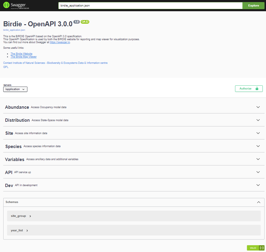
The endpoints are grouped as follows:
To make a simple request, follow these steps:
1. Expand the GET /openapi/v1/ramsar_sites - Get the RAMSAR sites info
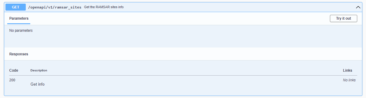
2. Click Try it out
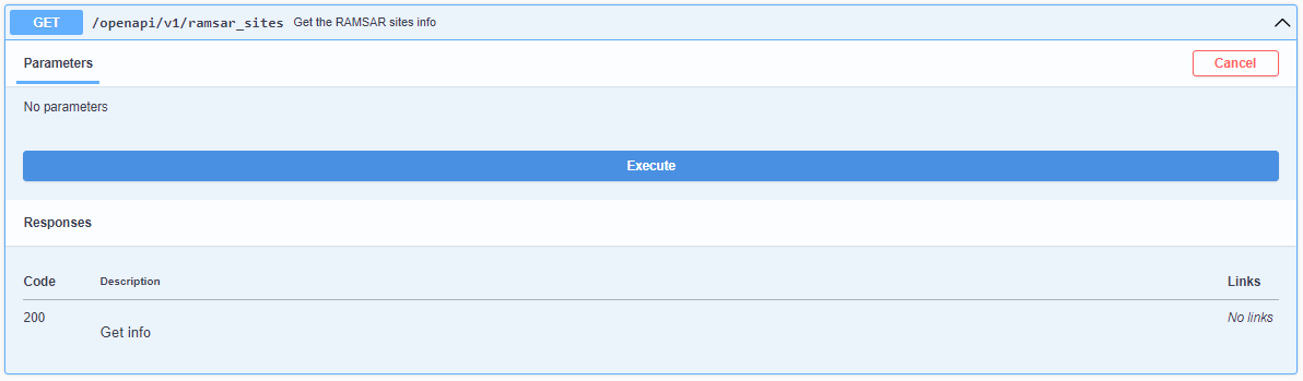
3. Click Execute. You should see your query results returned in the Response section.
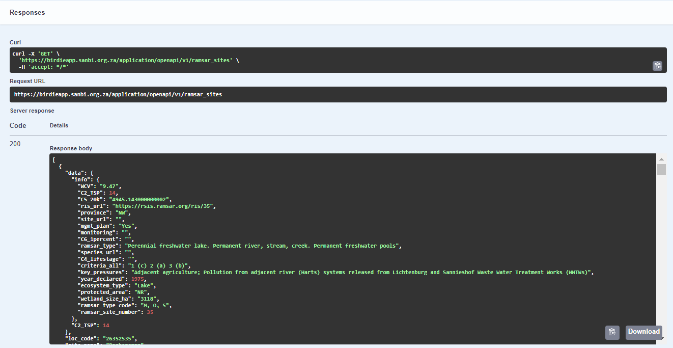
4. You can download these results by clicking on the ‘Download’ button. The results are downloaded as a .json file.
5. Alternatively, you can also use this API endpoint as a URL:

https://birdieapp.sanbi.org.za/application/openapi/v1/ramsar_sites
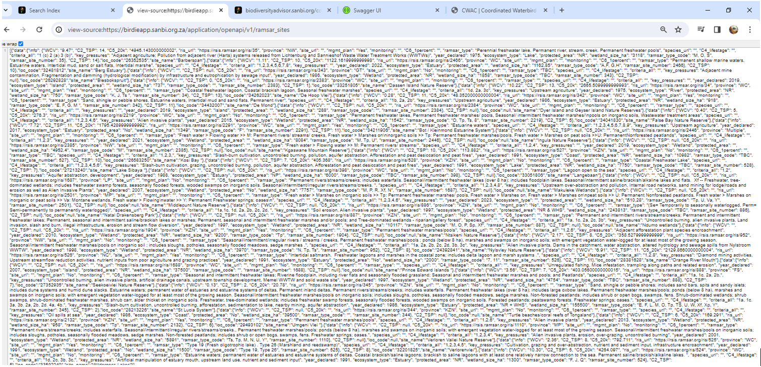
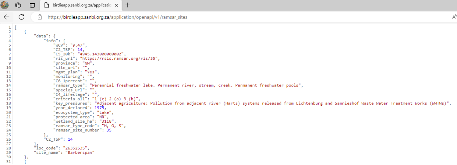
6. Recommedation: It’s best to copy and paste the url into Microsoft Edge. Microsoft Edge comes with a built-in feature that automatically formats JSON files, making it easier to understand.
JSON file viewed in Chrome *without* any extensions:
Same file viewed in Microsoft Edge:
Now let's make another request:
1. Expand the GET/openapi/v1/season_est_sites/{sites}/{species}/{season}/{start_year}/{end_year} -Get modelled estimates on species at site, over a range of years.
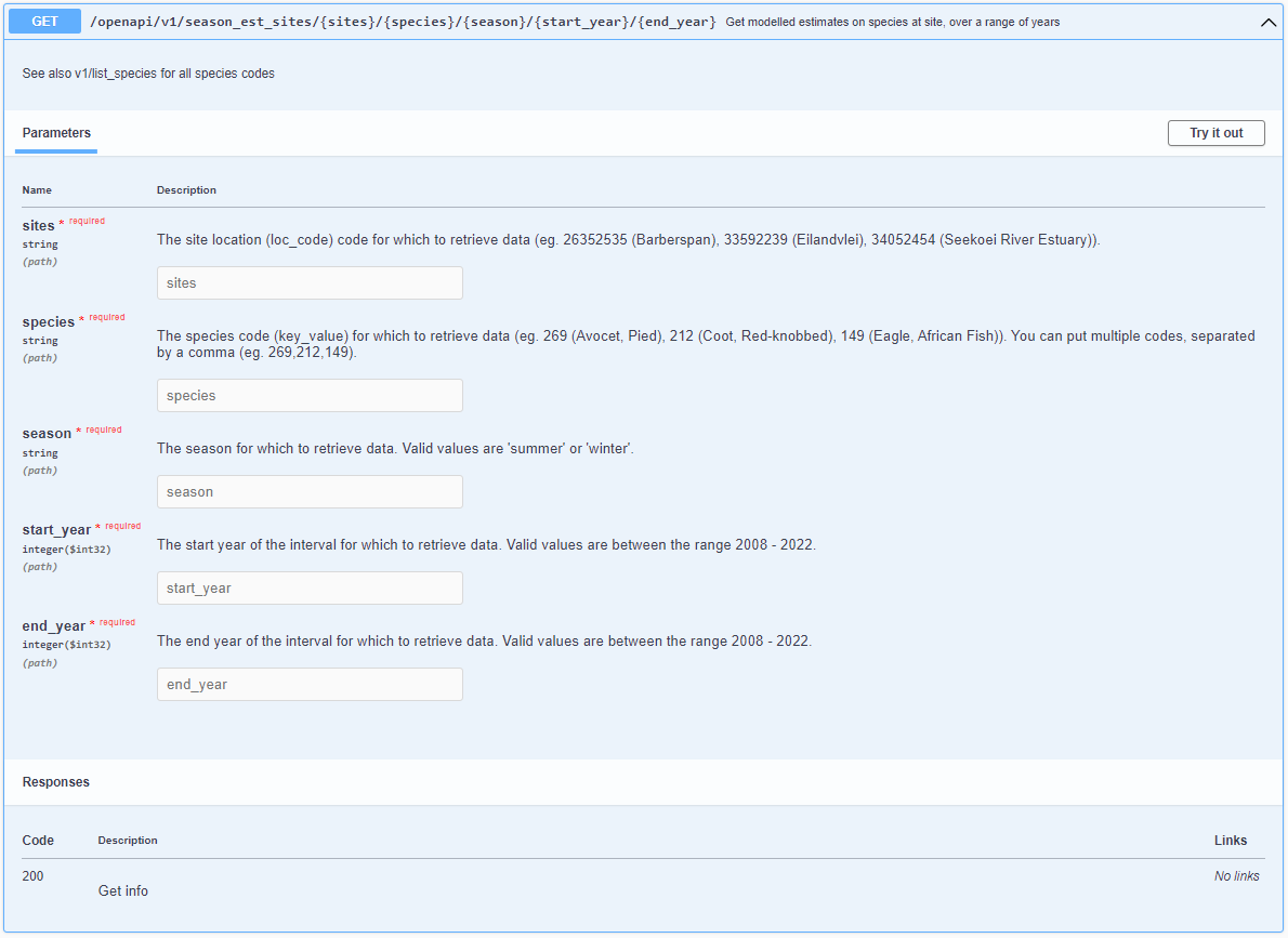
2. Click Try it out, so you can fill in variables in the different fields.
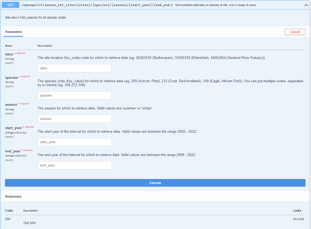
3. Enter the correct variables in the different fields. For each variable, there is a suggestion of what you can enter in each field. If you want different IDs, use the other endpoints to check the value (eg. GET/openapi/v1/list_species to get the list of species used, GET/openapi/v1/year_list to get the list of years).
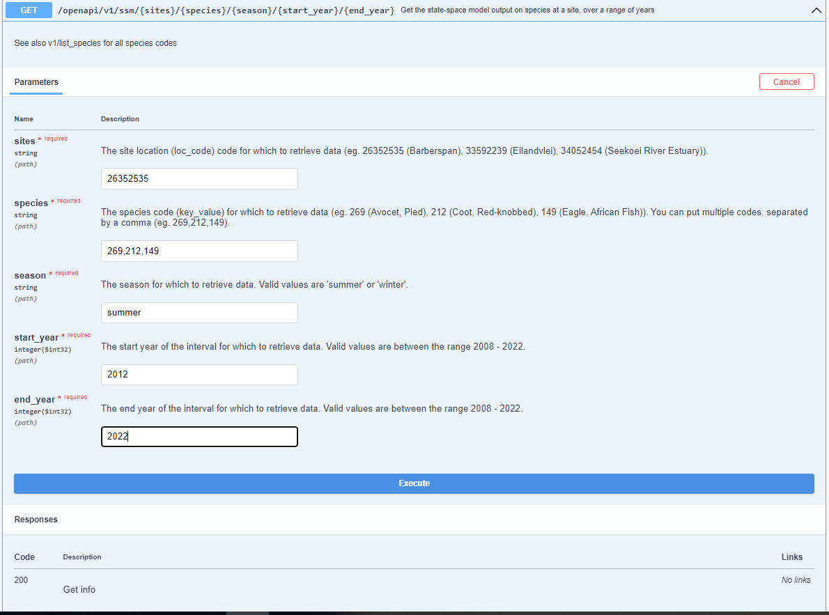
4. Click Execute. You should see your query results returned in the Response section.
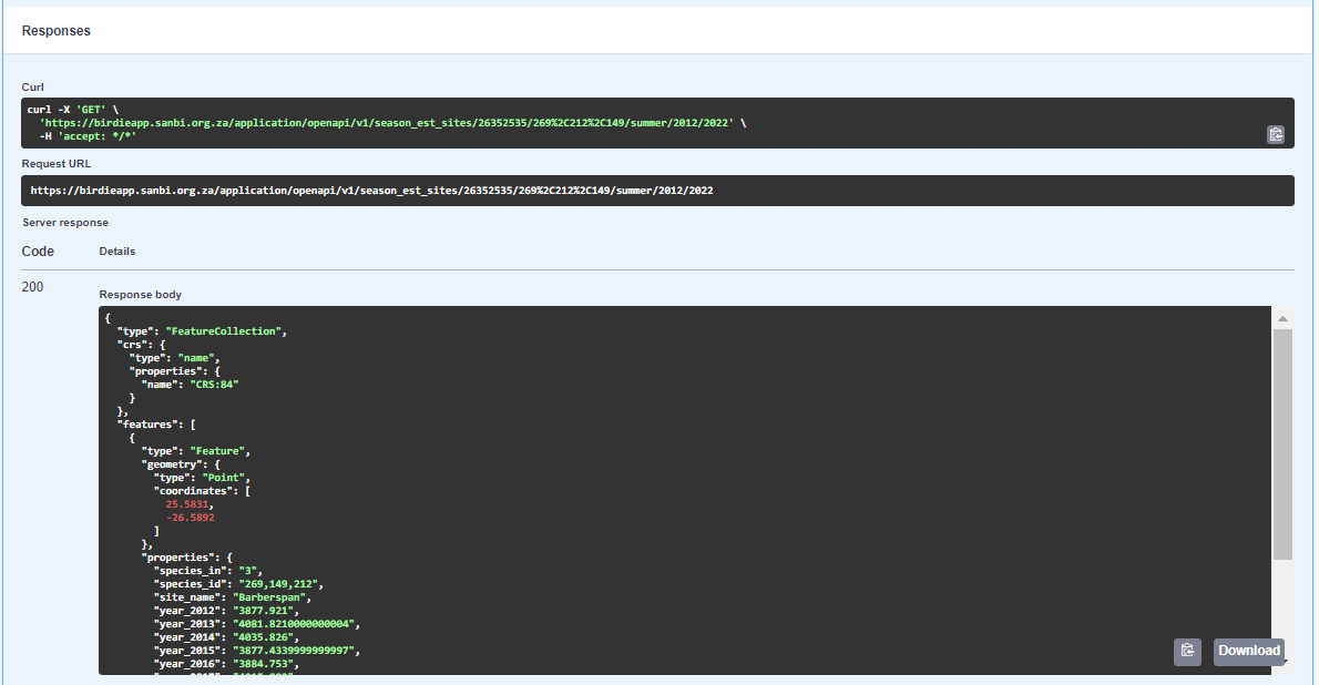
5. You can download these results by clicking on the ‘Download’ button. The results are downloaded as a .json file.
6. Alternatively, you can also use this API endpoint as a URL:

https://birdieapp.sanbi.org.za/application/openapi/v1/season_est_sites/26352535/269%2C212%2C149/summer/2012/2022
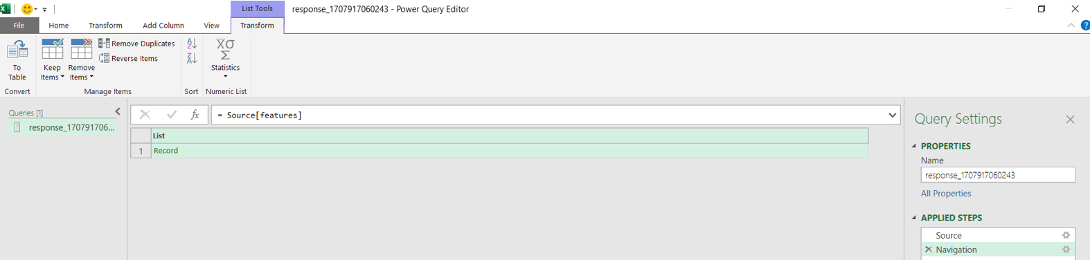
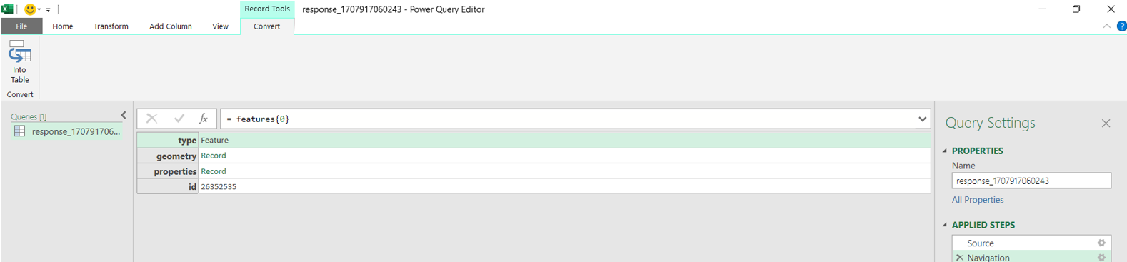
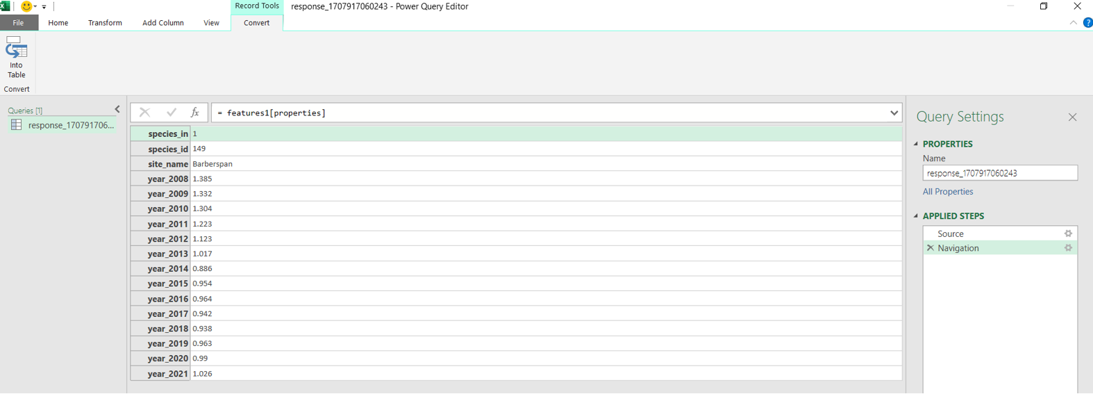
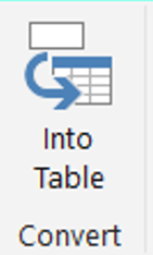
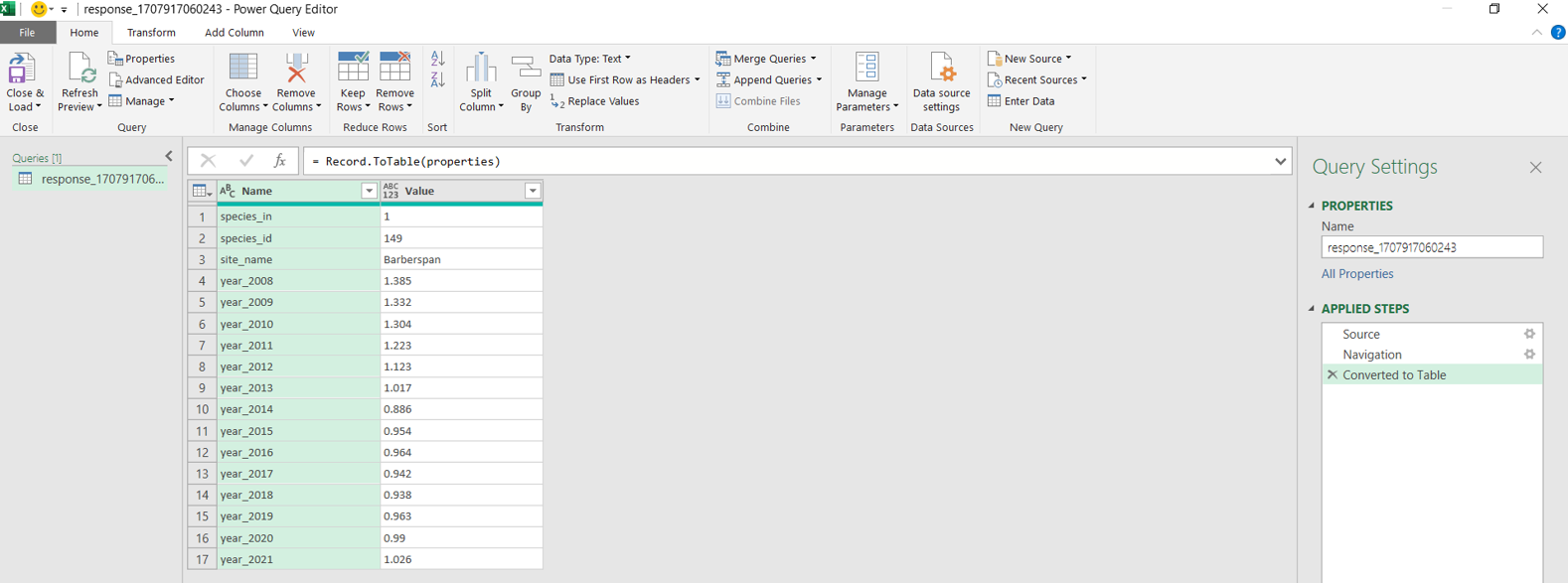
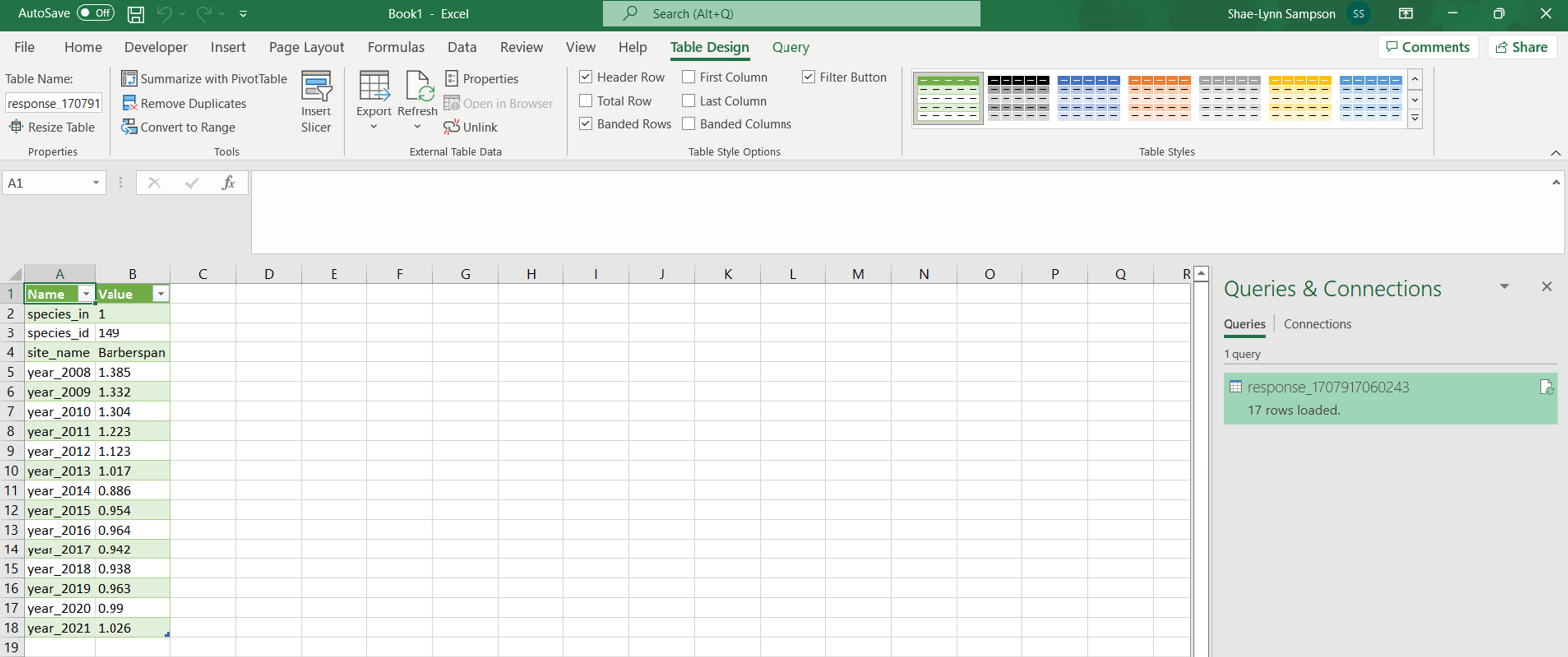
The results of queried data are returned as a URL. Users can download the queried data as JSON or GeoJSON files. JSON or GeoJSON files are text-based, lightweight interchange data formats that are used to share GIS data between systems. These files can be converted into csv or Excel using R or Excel.

install.packages("RJSONIO") library("RJSONIO ") Response_Barberspan <- fromJSON(“https://birdieapp.sanbi.org.za/application/openapi/v1/ratio_est_sites/26352535/149/PROP/2008/2022 ”) barberspan_prop <- Response_Barberspan[["features"]][[1]][["properties"]] table<- as.data.frame(barberspan_prop)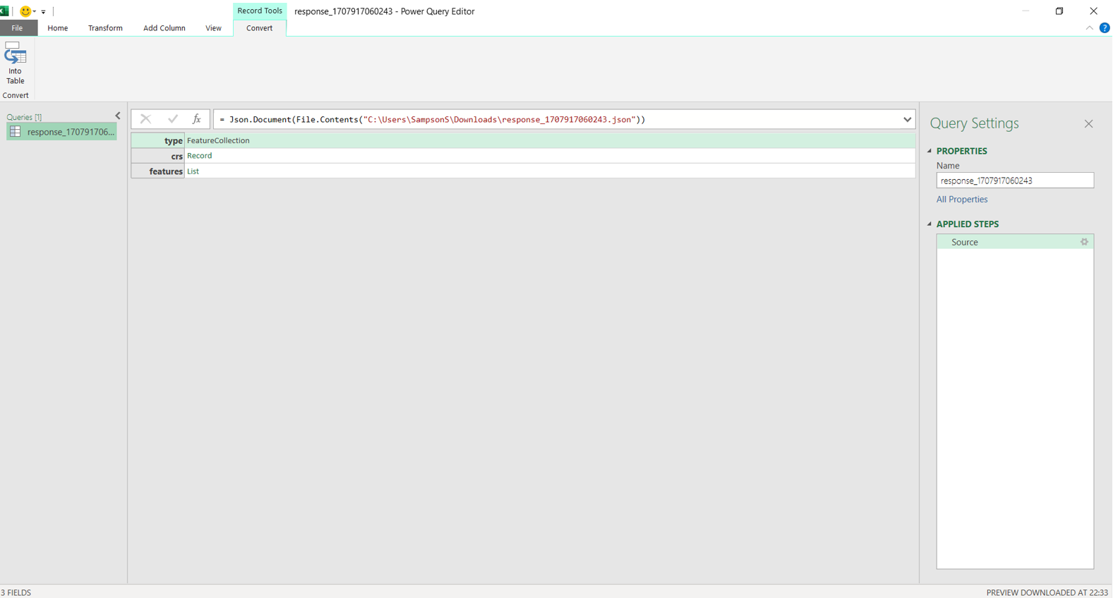
API (Application Programming Interface): A set of definitions, protocols, and tools for building software applications. APIs allow different systems to interact with each other programmatically.
API documentation: Documentation that describes how an API works so that data scientists can understand and use it. Usually includes reference documentation, tutorials, code samples, and overviews.
OAS: Abbreviation for OpenAPI specification.
OpenAPI (Swagger): A specification for describing REST APIs that can be used to generate interactive documentation, code libraries, and more.
REST API: An API that follows REST (Representational State Transfer) principles by exposing resources through endpoints that can be interacted with using standard HTTP methods like GET, POST, PUT, and DELETE. REST APIs return data in easy-to-process formats like JSON.
Swagger: A framework for the OpenAPI specification that includes a suite of tools for auto-generating documentation, client SDK generation, and more. In contrast to the term OpenAPI, Swagger now refers to API tooling related to the OpenAPI spec. Some of these tools include Swagger Editor, Swagger UI, Swagger Codegen, SwaggerHub, and others. These tools are managed by Smartbear. Note: Although ‘Swagger’ was the original name of the OpenAPI spec, the name was later changed to OpenAPI to reinforce the open, non-proprietary nature of the standard. OpenAPI is still often referred to as Swagger.
Swagger UI: An open-source web framework (on GitHub) that parses an OpenAPI specification document and generates an interactive documentation website. Swagger UI is the tool that transforms your spec into the BIRDIE OpenAPI.
Abundance: Abundance of a species refers to the number of individuals of that species at a site.
Area of Occupancy (AOO): Extension of the area occupied by a species in a given year.
Credible interval: We are 95% confident that the true value lies in this interval. The credible interval reflects the uncertainty around the estimate. Credible intervals are similar to confidence intervals; the former are used in Bayesian analyses (like here) and the latter are used in frequentist analyses. We are using 95% credible intervals, which means we are 95% confident that the true value lies in this interval. A wide credible interval means a lot of uncertainty whereas a narrow confidence interval reflects little uncertainty.
Distribution: The distribution of a species is the area over which it occurs.
Estimate: Our best guess at the true value of a parameter (quantity of interest) based on the observed data and a statistical model. It corresponds to the mean of the distribution of possible values provided by our model. Estimates come with a measure of uncertainty. In our case, this is a credible interval. A wide credible interval means there is a lot of uncertainty about the parameter.
Estimated occurance: The probability of occurrence of a species based on environmental covariates.
Guild: A guild refers to a grouping of species or species groups based on shared or similar traits such as diet, migratory status and/or taxonomy/morphology. Feeding guilds can be divided into herbivores (birds that have preference for or feed exclusively on plant and other vegetable matter), invertebrate feeders (birds that have preference for or feed exclusively on invertebrates including insects), piscivores (birds that have preference for or feed exclusively on fish). Migratory status refers to the overall general status of a species in a specified geographical location and is broadly divided into resident versus migratory species. Resident species include those that are largely restricted to a specific region in which it breeds and does not migrate or undertakes localised movements within the region or migratory (undertakes repeated, usually annual long- to medium movements to and from a specified region that are predictable in space and time; may or may not include breeding activity). Birds can be placed exclusively into one guild or multiple guilds (e.g. migrant species that feed exclusively on invertebrates).
Median: The value that cuts a distribution in half, such that if we picked one value randomly, we would have an equal chance of picking a value above as we would have picking value below the median.
Predicted occurance: The probability of occurrence taking into account the sampling effort at a specific site.
Species richness: The number of species that occur at a site.
Total population size: The total number of individuals estimated across all CWAC sites.